Hi, I’m Charlie Vorbach.
I teach cars to drive at NVIDIA. I’m interested in large-scale imitation and reinforcement learning.
Posts
-
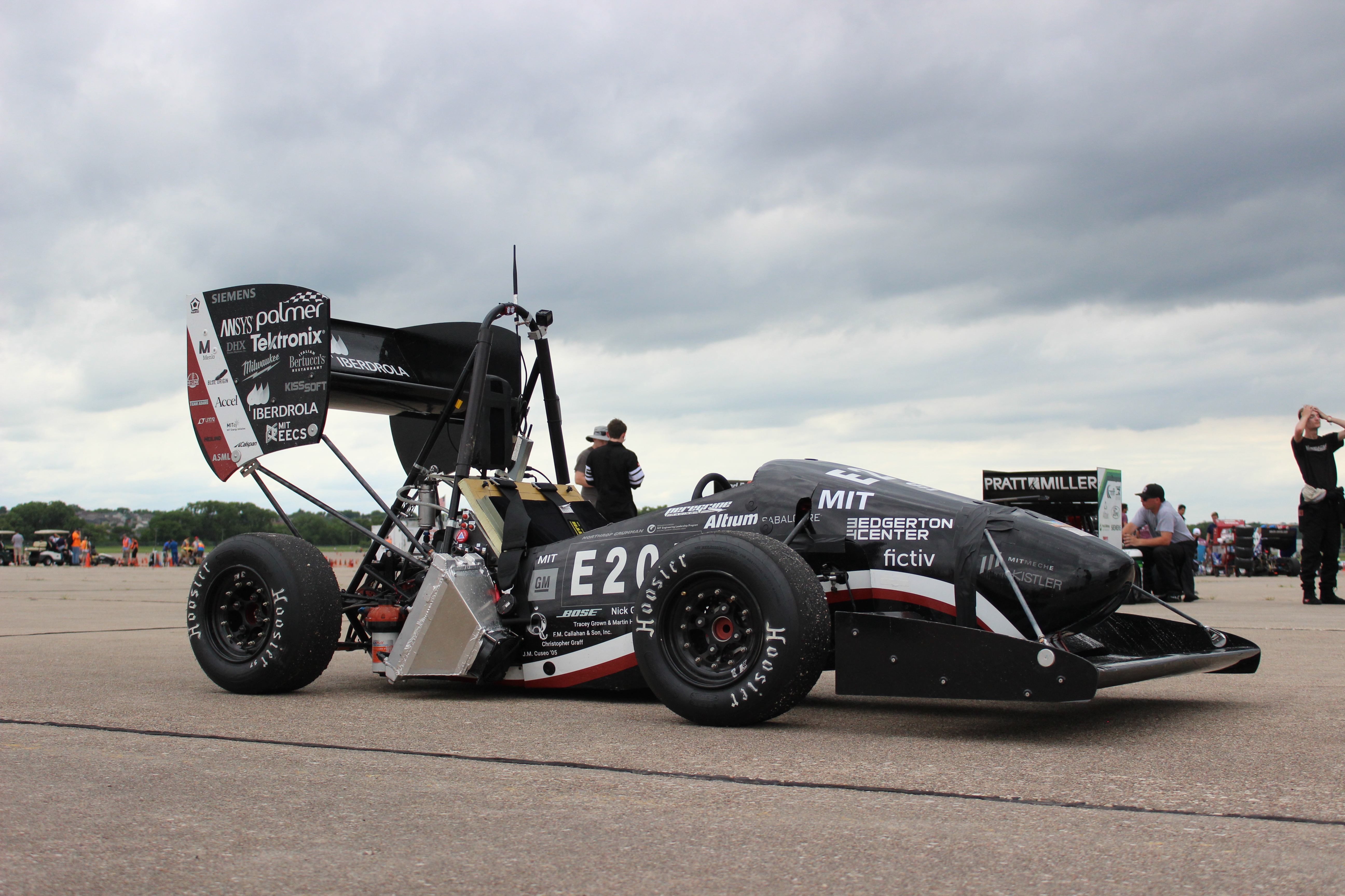
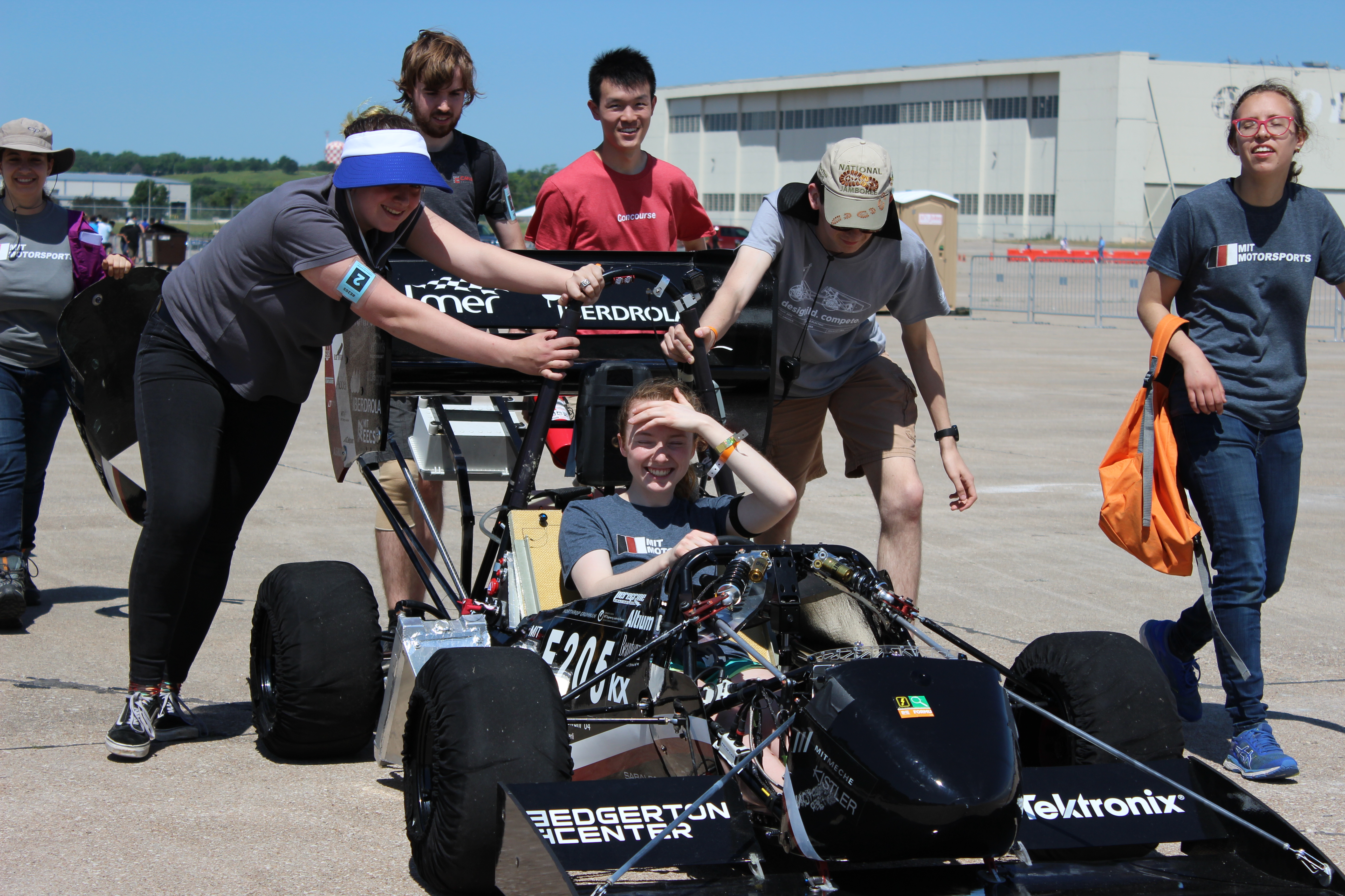
FSAE Lincoln Photos
I just wanted to share some photos from MIT Motorsports trip to Formula Student Lincoln. It was a crazy week of last-minute fixes and long hours on the car. Working with an amazing team made it fun and unforgettable.

-
Going Fast, But Not Too Fast
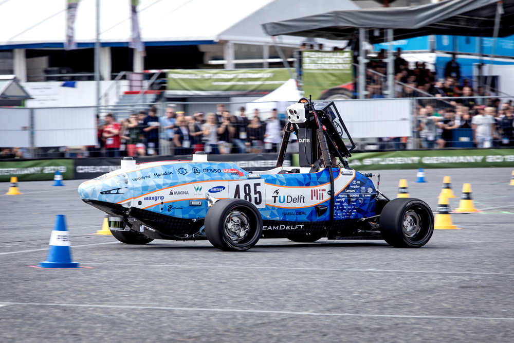
MIT Driverless/Delft MY2019 Car
MIT Motorsports's MY2019 Car Welcome back folks!
Leaves are turning, midterms are looming, and that means racecar is back in session. This year I’m excited to be work on MIT Motorsports FSAE Electric Racecar and to join Formula Student Driverless for their second year of collaboration with DUT Delft.
MIT Driverless is a really exciting project and I definitely plan to have updates on my vehicle modelling and controls work with them. For the moment though, I really want to document my power limiting work for Motorsports’s Electric team.
“What is power limiting,” you ask. “Don’t you want to use more power?” More power is more acceleration is faster lap times. A major goal of the team this year is to increase the rms power output from 15 kW to 25 kW. This requires a big technical leap to liquid battery cooling and is an exciting project for the battery team.
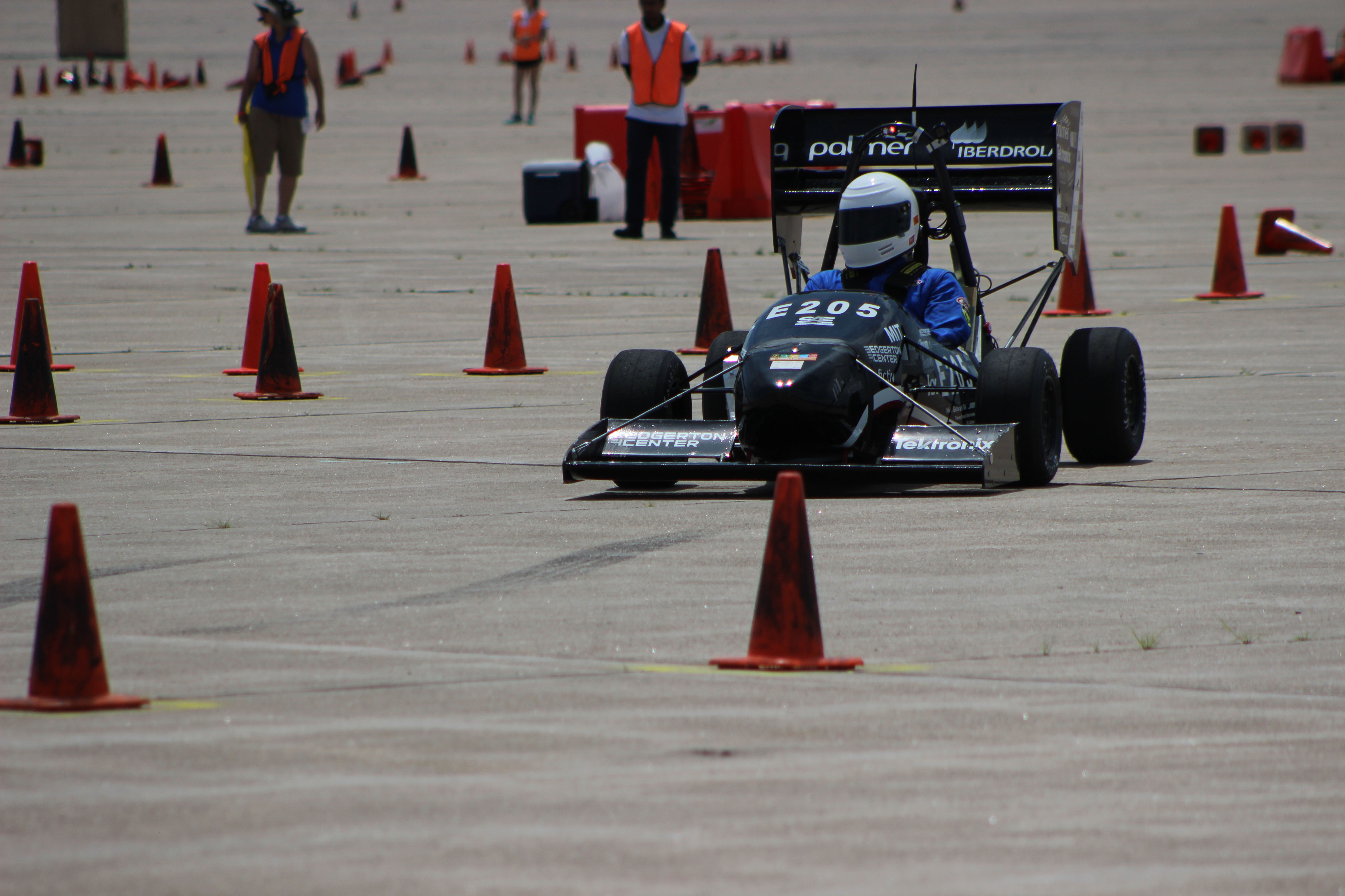
My job is to limit peak power. Our rules require us to draw no more 80 kW from the battery. At competition, the EE judge Dan Bocci actually installs a custom e-meter into the high voltage system to monitor compliance. In 2018, our racecar exceeded the limit for about 5 milliseconds off the line - enough to get us dequeued from the endurance event. It was real blow to the points total that year.
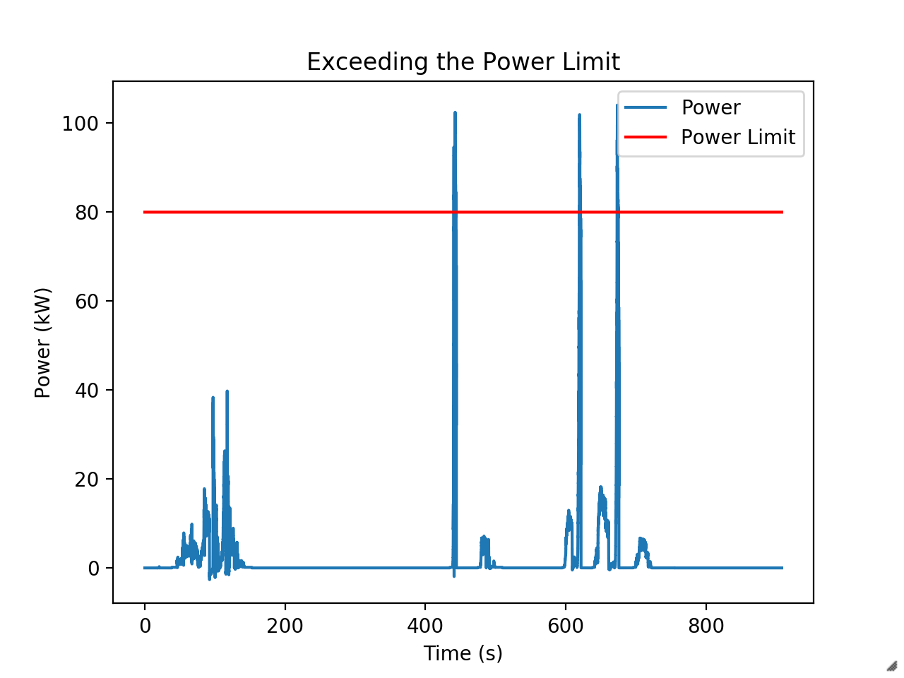
Little over the limit in this run. They’ve since changed the rules to just add a minute penalty, but limiting power is still required to have a competitive car. Our unlimited runs with the 2019 car have shown it will happily use more than 100 kW during acceleration if we let it. During competition we had to limit the driver’s maximum torque command by about a third to prevent exceeding the power limit. This was a big performance hit.
I’m responsible for implementing a better solution this year - one which only limits torque as necessary. The mechanical engineers in the audience might already have an idea for a strategy.
We can compute mechanical power, $ P = \tau \cdot \omega $, right? And we know motor speed from the Emrax motor’s resolver. So can’t we just limit torque, $ \tau = \frac{P}{\omega} $ such to never exceed 80 kW? There could be some inaccuracies from variation in motor efficiency over the torque-speed curve, but nothing a dynometer test and look-up table won’t solve.
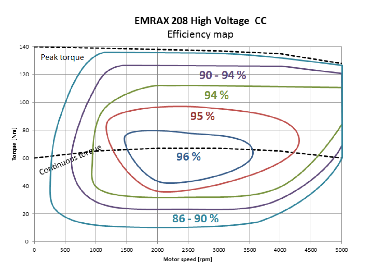
An untrusted estimate of the motor's map The issue with this strategy is that we’ve not yet been able to successfully run a dynometer test and that it difficult to estimate the actual torque (and therefore efficiency) produced while driving.
We use a Rinehart motor controller. It is a very nice, very fancy machine which has been the bane of three power limiting leads. The inverter introduces many quirks that make predicting efficiency harder.
The Rinehart has its own internal control loop which converts a torque command to a $I_q$ target for field-oriented control. It then does PID control to track this target. This introduces the problem that the Rinehart usually isn’t producing exactly the torque you are commanding. If you try to later try to calculate efficiency using recorded electrical power, torque command, and resolver speed you’ll get incorrect inefficiencies. This includes efficiencies which are greater than $1$ or less than $0$ because frequently the vehicle won’t be producing as much torque as you are commanding. Part of this is just the traction limit of the car.
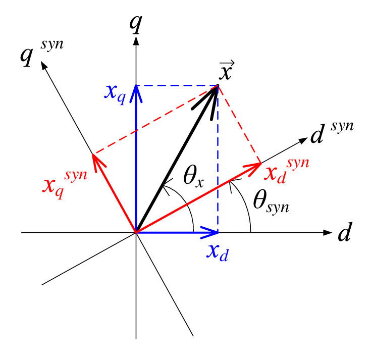
Field Oriented Control The Rinehart does give us a measurement called feedback torque which uses $I_q$ to produce a prediction of how much torque. However, this prediction is based on a linear relationship between $I_q$ and torque, when the relationship is non-linear. We could try to back out torque for ourselves using $I_q$ but it is hard to be confident of your results.
Field weakening introduces another level of complexity. Motor and generators are essentially the same device and so spinning a motor generates a back-emf proportional to speed. When this back-emf equals your bus voltage, you’ve reached the motor’s maximum speed and can’t command any more torque. The Emrax’s max speed with our battery voltage is less than the speeds we could see while driving and less than the thermal and mechanical speed limits of the motor. To command torque at higher speeds we use the Rinehart to produce $I_d$ current and produce torque over what would be the speed limit.
Field weakening is the decaying torque portion of this graph However, field weakening greatly reduces efficiency since $I_d$ current doesn’t produce torque. The onset of field weakening is depends on voltage which can sag and which changes as the battery is drained. This adds a third dimension to our lookup table.
If we want to run with different amounts of $I_d$ current (which we sometimes do) or control temperature you could need to add even more dimensions. The amount of data required and size of your lookup table quickly becomes impractical.
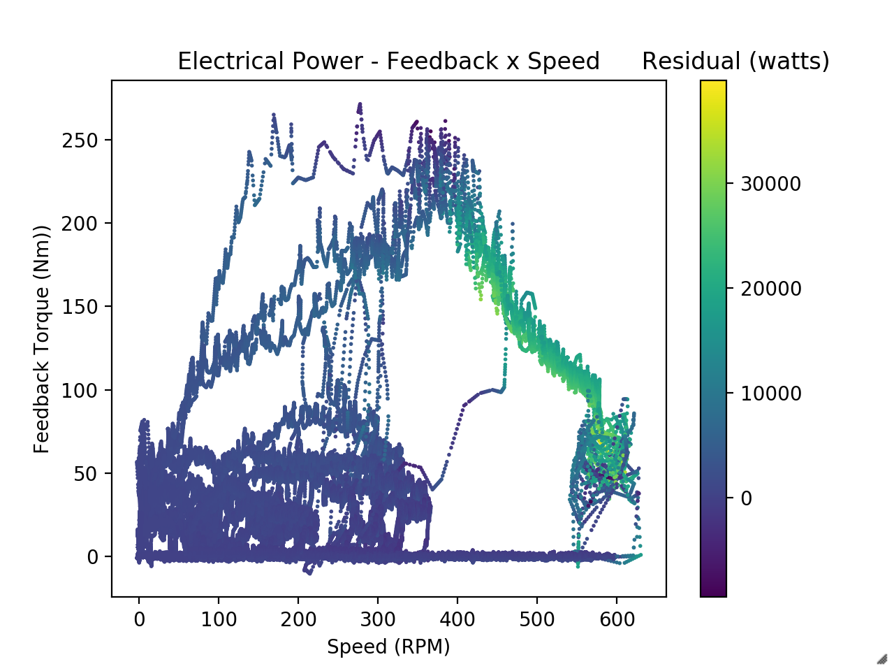
We’ve done a fair bit of analysis using just feedback torque and speed, but I think the way we’ll ultimately resolve this either by finally running a dynometer test or by using the magnetoelastic torque sensor we’re adding to model year 2020’s drivetrain to measure actual torque.
We use jupyter notebooks for data processing. Here’s the link to the live-hosted repository.
-
Low voltage, but HIGH PERFORMANCE!
I don’t have time for a big update, but I wanted to share my work on MIT Motorsport’s 2019 electric racecar’s low voltage management system. It isn’t anything too spicy, but I thought it was a fun project.
Anyway, here it is: LV Battery Management
-
Differentiating your filter
I wanted to write up a really cool derivative filter that I got to implement on the 2019 year car. Since I’m responsible for torque vectoring with the car’s wheel hub motors (Shameless plug for future post), I’m doing a lot of sensor work. So far though, this is been the coolest project.
There is a straightforward approach to take the derivative of a discrete signal. If you skip the subtlety of how derivatives analogize to a discrete signals, you could just say something like $ \frac{d}{dt} x[i] = \frac{x[i]-x[i-1]}{\Delta t} $ . For a pure signal this actually works great. It has minimal phase lag, is causal (real-time), and only requires keeping track of the two most recent values in the signal. If you’re clever you can sample at a constant frequency which removes the time dependence and makes it an LTI system. Slightly more sophisticated techniques like the five-point stencil method work similarly.
The difficulty arises when we introduce higher frequency noise. The z-transform of the transfer function is $ H(z) = \frac{1 - Z^{-1}}{T} $ so the frequency response is $ H(e^{j\omega}) = \frac{1 - e^{-j\omega}}{T}$. Taking the magnitude gives the amplitude response. It is kind of weird.
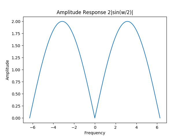
A key feature is that amplitude shrinks to zero for $\omega = 0$. This makes sense since the derivative of a constant signal should be zero. However, this also makes our system act like a high pass filter. It amplifies our higher frequency noise relative to the lower frequency signal.
There are many approaches to solve this issue, but we are looking for one that is simple to implement, fast, and has minimal phase lag. These properties are important since we use signals and their derivatives to make torque vectoring decisions. If the results are too laggy, then our torque vectoring controller won’t be responsive.
I found a paper Realtime Implementation of an Algebraic Derivative Estimation Scheme by Josef Zehetner, Johann Reger, and Martin Horn with a highly satisfactory method. I would recommend you read their paper for the full details. Essentially, we isolate a particular term in the Taylor series of the signal by applying a linear operator to a series ‘window’ of recent values. This method is nice since it only requires maintaining a circular buffer of the most recent samples. When we want to read the filter, we only need to sum a poylnomial function over each value in this window.
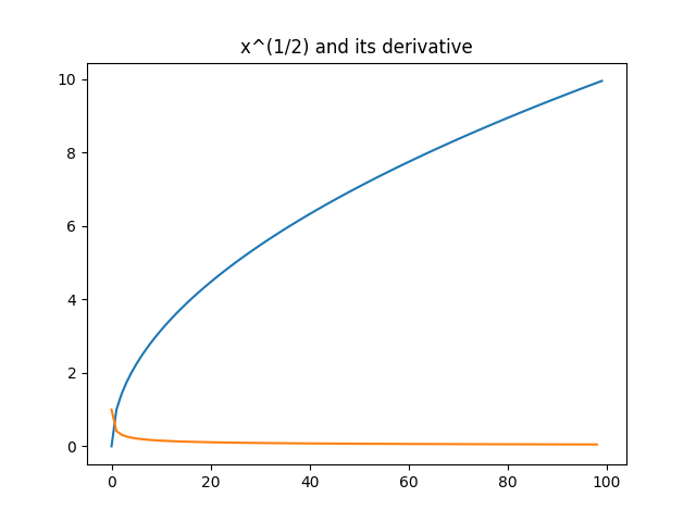
It works pretty good. Here is an example with $x[n] = \sqrt{n}$
Without any noise, our basic sequential difference method works well.
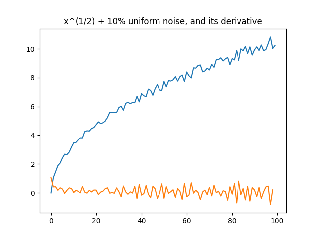
But once we add noise, it falls apart. You may notice that there is actually more noise in the derivative than the original signal.
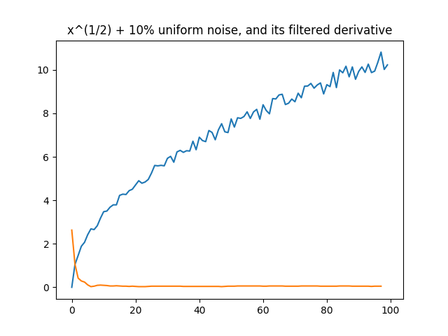
Our derivative filter comes to the rescue though. Other than some weirdness caused by the shortened window near the begining of the signal, it looks pretty good.
Just since they are real sweet, I might add some more plots of piecewise signals later. If you’d like to see the code for the filter you can find it here.
-
Open the pod bay doors, HAL Emulation
Hey-y’all! I wanted to share a real MIT FSAE project emulating the STM32f413’s HAL libraries. Our team switched from LPC to STM32 microcontrollers this year. We’ve also pushed to write many more unit tests and maybe even move toward automated build testing.
Our problem is that unit testing code for microcontrollers is hard. Our projects run on systems with very limited resources, restricted input/out, and dependent on the physical boards the microcontrollers are part of. This makes running tests on hardware slow, tricky to interpret, and hard to setup.
To show an example, the wheel speed sensing code I wrote for the car’s sensor nodes uses input capture interupts to measure quadrature encoded signals. The output speed is therefore dependent on values in specific GPIO registers and in a timer. Testing this code in hardware would require either feeding in known values through a testing rig or somehow replacing those calls with ‘TEST’ versions. This a recipe for too much work and/or messing preprocesor hacking. Not much fun.
I think the alternative we went with, native testing, is much better. Since our code is written in C, we have can compile it to run on our laptops like normal, non-embedded code. With a couple of additional targets added to our Makefile and judicious use of testing frameworks like Unity, we can quickly put together a powerful testing framework.
There are a couple of issues that need to be taken care of though. Firstly, our code uses constant global pointers which represent memory-mapped peripherals on the STM32. While our tests will compile, when we run them they will try to access unallocated memory locations and immediately throw a segmentation fault or worse.
While this seems like a bad problem, STM’s Hardware Abstraction Layer libraries provide a solution. Since they encapsulate the details of accessing physical registers and other peripherals, we can create a mocked version of these with allocated memory for native emulations of hardware locations.
That is exactly what I did in this project. I ripped out the hardware basis of the STM32F413’s HAL and CMSIS libraries and replaced it with an emulated version.
Its important to note that this allows our tests to compile and run, it doesn’t make hardware functions work - after all the hardware doesn’t exist when running natively. To let our programmers replace HAL functions with their own mocked version, I also declared them
__weak(we use gcc exclusively). I also started writing useful mock-ups of common functionality.This whole project is on github at stm32f4-hal-emulation.